Face Recognition - Eigen faces

We are going to create a basic facial recognition system using a technique called Principal Component Analysis. Its all math! This is a dimensionality reduction technique where we project the face images on the feature space which represents most of variance and insights of different faces. This face space is called Eigen Faces - eigen vectors of the set of faces.

Link to paper on Eigenfaces: (https://sites.cs.ucsb.edu/~mturk/Papers/mturk-CVPR91.pdf)

A must read paper, shows the real power of math and how even simplest of the concepts can be used to solve such a complex problem.

About the dataset:

The AT&T face dataset contains a set of grayscale face images with dimensions 92x112. The images are organized in 40 directories (one for each subject), which have names of the form sX, where X indicates the subject number (between 1 and 40). In each of these directories, there are ten different images of that subject, which have names of the form Y.pgm, where Y is the image number for that subject (between 1 and 10).

These 10 images per person are taken at different times, varying the lighting, facial expressions (open / closed eyes, smiling / not smiling) and facial details (glasses / no glasses). All the images were taken against a dark homogeneous background with the subjects in an upright, frontal position (with tolerance for some side movement).

Link: https://git-disl.github.io/GTDLBench/datasets/att_face_dataset/

Let's now import the dataset. First, download the zip file containing the dataset from the link above and then run the below code:

faces = {}
files_list = []

for path, subdirs, files in os.walk('.\ATnT'):
    for name in files:
        filename = str(os.path.join(path, name))
        if not filename.endswith(".pgm"):
            continue
            
        files_list.append(str(filename))
                
        with open(filename) as image:
            faces[filename] = cv2.imread(filename, cv2.IMREAD_GRAYSCALE)
            

'''
Each value in faces dictionary is a 2D numpy array. It is the image matrix for each image.
'''

Dataset is now imported. We'll perform EDA (Exploratory Data Analysis) to understand the data available before starting anything.

classes = set(filename.split("\\")[2] for filename in faces.keys())
print("Number of classes:", len(classes))
print("Number of images:", len(faces))

'''
Displaying images using image matrix for each image.
'''
fig, axes = plt.subplots(5,5, sharex=True, sharey=True, figsize=(6,8))
plt.gray()
face_images = list(faces.values())[-25:]

for i, axis in enumerate(axes.flat):
    axis.axis('off')
    axis.set_title(f'{files_list[i]}', fontsize=6)
    axis.imshow(face_images[i])
    
plt.show()

We'll split the data into training and testing set. We can use the train_test_split() from sklearn also, but we are doing it from scratch! We'll also flatten each image into a row vector and combines these row vectors to create training and test matrix.

We move 10th image of each class to test set. Thus, there are 40 images in test and 360 images in train. Now, we create matrices of each (train and test) by row vector of flattened image matrix. i.e. (112*92) === (10304*1)

original_faces = []  # matrix of column vector of each flattened image matrix (Train)
test_faces = []  # matrix of column vector of each falttened image matrix (Test)
face_labels = []  # just names of files (Train)
test_labels = []  # just names of files (Test)

for key,val in faces.items():
        
    if '10.pgm' in str(key):
        test_faces.append(val.flatten())
        test_labels.append(key)
        continue
    
    original_faces.append(val.flatten())
    face_labels.append(key)
    
# Create original_faces as (n_samples,n_pixels) matrix
print("Training data: ")
original_faces = np.array(original_faces)
print(original_faces)
print(original_faces.shape)

print("\nTest data: ")
test_faces = np.array(test_faces)
print(test_faces)
print(test_faces.shape)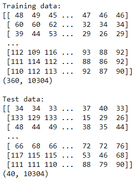

Before starting with code, let's first understand the math we'll be using here.

Eigenvalues and Eigenvectors:

An eigenvector of a square matrix A is a non-zero vector x that satisfies the equation:

A x = λ x

where λ is a scalar, called the eigenvalue associated with x. In other words, when A is multiplied by x, the result is a scaled version of x, where the scaling factor is λ.

To find the eigenvalues and eigenvectors of a matrix, we can solve the following equation:

det(A - λ I) = 0

where det(A - λ I) is the determinant of the matrix A - λ I, and I is the identity matrix of the same size as A. The solutions to this equation are the eigenvalues of A. Once we have found the eigenvalues, we can find the eigenvectors by solving the equation:

(A - λ I) x = 0

for each eigenvalue λ. The nonzero solutions to this equation are the eigenvectors corresponding to λ.

Geometrically, eigenvalues and eigenvectors represent the scaling and directionality of linear transformations.

Principal Component Analysis:

PCA (Principal Component Analysis) is a dimensionality reduction technique that uses eigenvectors and eigenvalues to transform a dataset into a new coordinate system, where the data can be visualized or analyzed more easily.

The main idea behind PCA is to find the principal components of the dataset, which are the directions along which the data varies the most. To do this, PCA finds the eigenvectors and eigenvalues of the covariance matrix of the data.

First, we standardize the data and find the covariance matrix. The covariance matrix is a square matrix that describes the covariance between pairs of variables in the dataset.

X_std = (X - mean(X)) / std(X)

Cov = (1/n) * X_std ^T * X_std

where X is the dataset, mean(X) is the mean of all the variables, std(X) is the standard deviation of all the variables, X_std^T is the transpose of X_std, and Cov is the covariance matrix (p x p).

The eigenvectors and eigenvalues of covariance matrix provide information about the most important directions of variation in the data. The eigenvectors are the principal components of the data, and they represent the directions along which the data varies the most. The corresponding eigenvalues represent the amount of variation in the data that is explained by each principal component.

The eigenvectors and eigenvalues of the covariance matrix can be computed using a variety of methods, including the power iteration method or the singular value decomposition (SVD) method.

U, S, V^T = svd(Cov)

where U is the matrix of eigenvectors, S is the diagonal matrix of eigenvalues, and V^T is the transpose of the matrix V.

PCA selects the top k eigenvectors with the largest eigenvalues, and uses them to transform the data into a new coordinate system where each axis represents a principal component. This new coordinate system is chosen so that the data is as spread out as possible along the new axes, with the first axis representing the direction of maximum variance, the second axis representing the second direction of maximum variance, and so on.

By projecting the data onto the new coordinate system, we obtain a lower-dimensional representation of the data that retains as much of the original variation as possible. This can be useful for visualizing the data or for reducing the number of features in a machine learning problem.

Y = X _std* U_k

where X_std is the standardized data matrix, U_k is the matrix of the top k eigenvectors (columns) of U, and Y is the matrix of transformed data in the new coordinate system (n x k).

Let's now see how PCA and Eigenfaces can be implemented.

def principalComponentAnalysis(X, n_components=None):
    
    if n_components is None:
        n_components = X.shape[1]
    
    X_mean = np.mean(X, axis=0)
    X_standard = X - X_mean
    X_cov = np.cov(X_standard, rowvar=True)

    eigen_values, eigen_vectors = np.linalg.eigh(X_cov)
    sorted_order = np.flip(np.argsort(eigen_values))
    eigen_values = eigen_values[sorted_order]
    eigen_vectors = eigen_vectors[:, sorted_order]

    components = eigen_vectors[:, :n_components]
    X_pca = np.dot(X_standard.transpose(), components)
    eigen_faces = np.dot(X_pca, components.transpose()).transpose()

    return X_pca, components, eigen_faces, X_mean

We are now ready to understand the main concept here :

Eigen Faces

Eigenfaces is a popular technique used in computer vision and facial recognition to represent a set of face images in a lower-dimensional space. The technique uses principal component analysis (PCA) to find the most important features in the face images and represent them as a set of eigenvectors.

The eigenvectors, also called eigenfaces, form a basis for the original face images, which can be reconstructed from linear combinations of the eigenfaces.

Now let's start reconstructing the images using Eigenfaces as discussed above.

Image Reconstruction

Let's reconstruct image after reducing the dimensionality i.e. trying with different number of principal components.

def imageReconstruction(original_faces, eigenfaces, faceshape, idx, 
                       face_labels):

    # plot the original image and the reconstructed image
    fig, axes = plt.subplots(1,2,sharex=True,sharey=True,figsize=(8,6))
    plt.gray()

    axes[0].axis('off')
    axes[1].axis('off')

    axes[0].imshow(original_faces[idx].reshape(faceshape))
    axes[0].set_title(f'Original {face_labels[idx]} image')
    axes[1].imshow(eigenfaces[idx].reshape(faceshape))
    axes[1].set_title(f'Reconstructed {face_labels[idx]} image')

    plt.show()
    
    
n_components = 100
X_pca, components, eigenfaces, X_mean, mse = principalComponentAnalysis(original_faces, n_components)
imageReconstruction(original_faces, eigenfaces, faceshape, 0, face_labels)
imageReconstruction(original_faces, eigenfaces, faceshape, 1, face_labels)

The above result is obtained with n = 100. This can be tried with different number of principal components. More the principal components, the reconstructed image is more clear.

Mean Face

Mean face represents the mean vector of original data. It is computed by taking the mean along with each feature/column of input data.

fig, axes = plt.subplots(1,1,sharex=True,sharey=True,figsize=(6,4));
plt.gray();

axes.axis('off');
axes.imshow(X_mean.reshape(faceshape));
axes.set_title("Mean face");

Face Recognition Model

Now let's code up a model which implements the face recognition based on the concepts learned above.

def model(input_image, eigenfaces, X_mean, original_faces):
    # Calculate weights for original images
    weights = eigenfaces @ (original_faces - X_mean).T

    # Test sample images
    query = faces[input_image].reshape(1,-1)
    query_weight = eigenfaces @ (query - X_mean).T

    euclidean_distance = np.linalg.norm(weights - query_weight, axis=0)

    best_match = np.argmin(euclidean_distance)
    print(f"Error Value (Euclidean distance) = 
                                   {euclidean_distance[best_match]}")

    # Visualize test result
    fig, axes = plt.subplots(1,2,sharex=True,sharey=True,figsize=(4,2))
    plt.gray()

    axes[0].axis('off')
    axes[0].imshow(query.reshape(faceshape))
    axes[0].set_title(f"Query {input_image}", fontsize=8)
    axes[1].axis('off')
    axes[1].imshow(original_faces[best_match].reshape(faceshape))
    axes[1].set_title(f"Best match {face_label[best_match]}", fontsize=8)

    plt.show()
   
"""
Iterate through all the images in the test data and 
test the accurate by taking different number of components
"""

for i in range(0, len(test_labels)):
    model(test_labels[i], eigenfaces, X_mean, original_faces)

Overall, the model function performs face recognition by computing weights for the original images and comparing the weights of a test image with the weights of the original images using Euclidean distance. It then visualizes the test result by showing the test image and the best matching image from the dataset.

Conclusion

Eigenfaces and PCA offer an effective approach for face recognition by reducing the dimensionality of face images and capturing the essential facial features. The article provides a comprehensive understanding of these techniques, covering the computation of eigenfaces, the application of PCA, and their implementation in a face recognition model. By using code snippets, readers gain practical insights into the underlying concepts and can apply them to their own projects in the field of facial recognition.

Eigenfaces and PCA does have a lot of disadvantages too and thus are currently not used extensively. They are replaced by Neural Networks. We'll will discuss this soon in the later posts.

Thanks for reading. Cheers!